Day 4. Understand what’s important

amp.posted_on

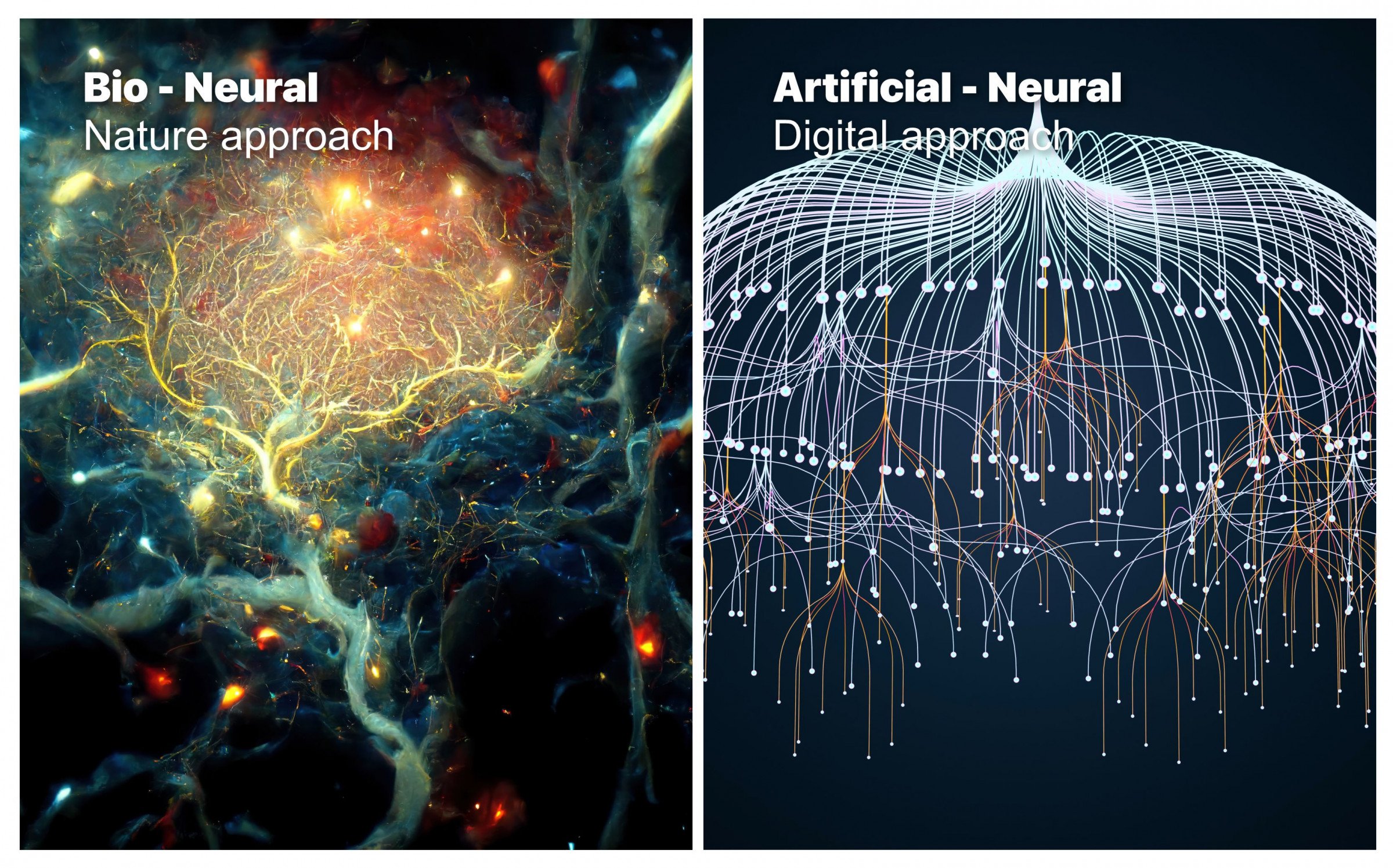
AI can be broken down into three main sub-processes: data, structure, and learning.

1. Data: The first step in developing an AI model is to provide the appropriate data. Depending on the type of mechanism being used, this may involve obtaining labeled data or implementing a system for providing feedback.

2. Structure: Once the data has been obtained, the next step is to create a structure for the neural network or any pre-processing and post-processing steps that may be necessary. This includes designing the architecture of the network, as well as any data preprocessing or feature engineering that may be required.

3. Learning: The final step is to train the system, maintain it, and apply some level of supervision. This includes implementing a learning algorithm, such as gradient descent, and adjusting the model's parameters as necessary to optimize performance. Additionally, it also includes maintaining the system by monitoring its performance, updating it with new data, and troubleshooting any issues that may arise.

Personally, I am not interested in creating large artificial neural networks (ANNs) and training them with massive datasets using excessive computational power. This is because companies like OpenAI have already achieved this and it would be difficult for me to compete with the vast resources they have at their disposal. The focus, instead, is on creating efficient and effective models using the available resources and finding creative ways to work with smaller datasets.

Articulate questions

Instead of focusing on creating large artificial neural networks (ANNs) and training them with massive datasets, my goal is to address some of the fundamental unanswered questions in the field of AI and AGI. Understanding these big questions is crucial before delving into the practical implementation of ANNs and attempting to deploy them in the real world.

Some of the key questions I am interested in exploring include:

Why do we need large datasets to train ANNs, when humans can learn from limited data?
How can we pre-train ANNs in a more efficient manner?
How can we expand an ANN from a single-task network to a multi-task and multi-modal network?
How can we make AI systems self-maintaining and self-progressive?

By focusing on these questions, I hope to gain a deeper understanding of the underlying principles of AI and AGI and contribute to the development of more advanced and capable AI systems.

Recently, I have been focusing on demonstrating how I can formulate hypotheses, implement them and test them in the real world, with the goal of potentially discovering or creating answers to some of the fundamental questions in the field of AI and AGI. I believe that this approach allows me to gain a deeper understanding of the underlying principles of AI and contribute to the development of more advanced and capable AI systems.

How start?

Let's simplify the process by using a camera as the data input, as it provides a vast amount of data and is relatively inexpensive. Instead of using pre-existing datasets, I will explore ways to train ANNs using images fed directly from the camera and using unsupervised learning methods. Then, I will use supervised methods to label certain groups. If you're interested in specific applications like face detection, finger gesture detection, image generation, or AI chat, there are plenty of resources available online that focus on these specific fields.

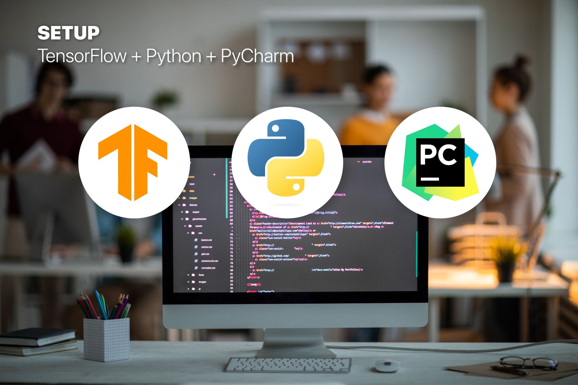
At this stage, I am using a camera as the data input, a PC with a Radeon VGA graphics card, PyCharm as the development environment, and some knowledge and understanding to test and experiment with the implementation.

Let's work on training a basic perceptron

Training a perceptron, which is a simple type of artificial neural network, involves several steps:

1. Initialize the weights: The first step is to initialize the weights of the perceptron. This is typically done by assigning random values to the weights.

2. Feedforward: The input data is then fed into the perceptron, and the dot product of the input and the weights is calculated. This value is then passed through an activation function, such as a step function or a sigmoid function, to produce the output of the perceptron.

3. Calculate the error: The difference between the predicted output and the actual output is calculated. This is known as the error.

4. Update the weights: The weights are then updated based on the error. This is typically done using gradient descent, which adjusts the weights in the opposite direction of the gradient of the error with respect to the weights.

5. Repeat steps 2-4: The process is repeated for a number of iterations, until the error is minimized.

6. Test: Finally, the trained perceptron is tested on new unseen data to evaluate its performance.

%7B%22python%22%3A%22import%20tensorflow%20as%20tf%5Cnimport%20numpy%20as%20np%5Cnimport%20matplotlib.pyplot%20as%20plt%5Cn%5Cn%23%20Set%20up%20the%20data%20with%20a%20noisy%20linear%20relationship%20between%20X%20and%20Y.%5Cnnum_examples%20%3D%2050%5CnX%20%3D%20np.array(%5Bnp.linspace(-2%2C%204%2C%20num_examples)%2C%20np.linspace(-6%2C%206%2C%20num_examples)%5D)%5Cn%23%20Add%20random%20noise%20(gaussian%2C%20mean%200%2C%20stdev%201)%5CnX%20%2B%3D%20np.random.randn(2%2C%20num_examples)%5Cn%23%20Split%20into%20x%20and%20y%5Cnx%2C%20y%20%3D%20X%5Cn%23%20Add%20the%20bias%20node%20which%20always%20has%20a%20value%20of%201%5Cnx_with_bias%20%3D%20np.array(%5B(1.%2C%20a)%20for%20a%20in%20x%5D).astype(np.float32)%5Cn%5Cn%5Cn%23%20Keep%20track%20of%20the%20loss%20at%20each%20iteration%20so%20we%20can%20chart%20it%20later%5Cnlosses%20%3D%20%5B%5D%5Cn%23%20How%20many%20iterations%20to%20run%20our%20training%5Cntraining_steps%20%3D%2050%5Cn%23%20The%20learning%20rate.%20Also%20known%20has%20the%20step%20size.%20This%20changes%20how%20far%5Cn%23%20we%20move%20down%20the%20gradient%20toward%20lower%20error%20at%20each%20step.%20Too%20large%5Cn%23%20jumps%20risk%20inaccuracy%2C%20too%20small%20slow%20the%20learning.%5Cnlearning_rate%20%3D%200.002%5Cn%5Cn%23%20Set%20up%20all%20the%20tensors.%5Cn%23%20Our%20input%20layer%20is%20the%20x%20value%20and%20the%20bias%20node.%5Cninput%20%3D%20tf.constant(x_with_bias)%5Cn%23%20Our%20target%20is%20the%20y%20values.%20They%20need%20to%20be%20massaged%20to%20the%20right%20shape.%5Cntarget%20%3D%20tf.constant(np.transpose(%5By%5D).astype(np.float32))%5Cn%23%20Weights%20are%20a%20variable.%20They%20change%20every%20time%20through%20the%20loop.%5Cn%23%20Weights%20are%20initialized%20to%20random%20values%20(gaussian%2C%20mean%200%2C%20stdev%200.1)%5Cnweights%20%3D%20tf.Variable(tf.random.normal(%5B2%2C%201%5D%2C%200%2C%200.1))%5Cn%5Cn%5Cn%5Cn%23%20Set%20up%20all%20operations%20that%20will%20run%20in%20the%20loop.%5Cn%23%20For%20all%20x%20values%2C%20generate%20our%20estimate%20on%20all%20y%20given%20our%20current%5Cn%23%20weights.%20So%2C%20this%20is%20computing%20y%20%3D%20w2%20*%20x%20%2B%20w1%20*%20bias%5Cnyhat%20%3D%20tf.matmul(input%2C%20weights)%5Cn%23%20Compute%20the%20error%2C%20which%20is%20just%20the%20difference%20between%20our%5Cn%23%20estimate%20of%20y%20and%20what%20y%20actually%20is.%5Cnyerror%20%3D%20tf.subtract(yhat%2C%20target)%5Cn%23%20We%20are%20going%20to%20minimize%20the%20L2%20loss.%20The%20L2%20loss%20is%20the%20sum%20of%20the%5Cn%23%20squared%20error%20for%20all%20our%20estimates%20of%20y.%20This%20penalizes%20large%20errors%5Cn%23%20a%20lot%2C%20but%20small%20errors%20only%20a%20little.%5Cnloss%20%3D%20tf.nn.l2_loss(yerror)%5Cn%5Cn%23%20Perform%20gradient%20descent.%5Cn%23%20This%20essentially%20just%20updates%20weights%2C%20like%20weights%20-%3D%20grads%20*%20learning_rate%5Cn%23%20using%20the%20partial%20derivative%20of%20the%20loss%20with%20respect%20to%20the%5Cn%23%20weights.%20It's%20the%20direction%20we%20want%20to%20go%20to%20move%20toward%20lower%20error.%5Cnoptimizer%20%3D%20tf.optimizers.SGD(learning_rate)%5Cn%5Cn%23%20At%20this%20point%2C%20we've%20defined%20all%20our%20tensors%20and%20run%20our%20initialization%5Cn%23%20operations.%20We've%20also%20set%20up%20the%20operations%20that%20will%20repeatedly%20be%20run%5Cn%23%20inside%20the%20training%20loop.%20All%20the%20training%20loop%20is%20going%20to%20do%20is%5Cn%23%20repeatedly%20call%20run%2C%20inducing%20the%20gradient%20descent%20operation%2C%20which%20has%20the%20effect%20of%5Cn%23%20repeatedly%20changing%20weights%20by%20a%20small%20amount%20in%20the%20direction%20(the%5Cn%23%20partial%20derivative%20or%20gradient)%20that%20will%20reduce%20the%20error%20(the%20L2%20loss).%5Cnfor%20_%20in%20range(training_steps)%3A%5Cn%20%20%20%20with%20tf.GradientTape()%20as%20tape%3A%5Cn%20%20%20%20%20%20%20%20yhat%20%3D%20tf.matmul(input%2C%20weights)%5Cn%20%20%20%20%20%20%20%20yerror%20%3D%20tf.subtract(yhat%2C%20target)%5Cn%20%20%20%20%20%20%20%20current_loss%20%3D%20tf.nn.l2_loss(yerror)%5Cn%20%20%20%20grads%20%3D%20tape.gradient(current_loss%2C%20%5Bweights%5D)%5Cn%20%20%20%20optimizer.apply_gradients(zip(grads%2C%20%5Bweights%5D))%5Cn%5Cn%20%20%20%20%23%20Here%2C%20we're%20keeping%20a%20history%20of%20the%20losses%20to%20plot%20later%5Cn%20%20%20%20%23%20so%20we%20can%20see%20the%20change%20in%20loss%20as%20training%20progresses.%5Cn%20%20%20%20losses.append(current_loss.numpy())%5Cn%5Cn%5Cn%5Cn%5Cn%23%20Training%20is%20done%2C%20get%20the%20final%20values%20for%20the%20charts%5Cnbetas%20%3D%20weights%5Cnyhat%20%3D%20yhat%5Cn%5Cn%23%20Show%20the%20results.%5Cnfig%2C%20(ax1%2C%20ax2)%20%3D%20plt.subplots(1%2C%202)%5Cnplt.subplots_adjust(wspace%3D.3)%5Cnfig.set_size_inches(10%2C%204)%5Cnax1.scatter(x%2C%20y%2C%20alpha%3D.7)%5Cnax1.scatter(x%2C%20np.transpose(yhat)%5B0%5D%2C%20c%3D%5C%22g%5C%22%2C%20alpha%3D.6)%5Cnline_x_range%20%3D%20(-4%2C%206)%5Cnax1.plot(line_x_range%2C%20%5Bbetas%5B0%5D%20%2B%20a%20*%20betas%5B1%5D%20for%20a%20in%20line_x_range%5D%2C%20%5C%22g%5C%22%2C%20alpha%3D0.6)%5Cnax2.plot(range(0%2C%20training_steps)%2C%20losses)%5Cnax2.set_ylabel(%5C%22Loss%5C%22)%5Cnax2.set_xlabel(%5C%22Training%20steps%5C%22)%5Cnplt.show()%5Cn%22%7D

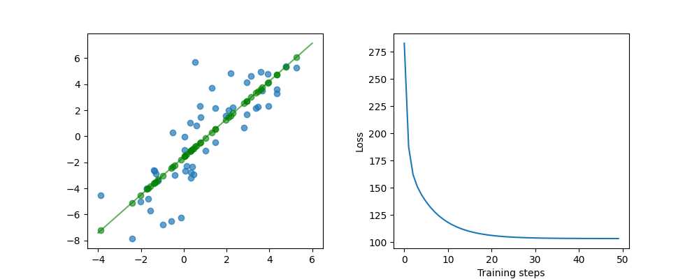
By utilizing the code provided, you will gain exposure to some basic and crucial concepts and libraries that will be utilized in the future AI/ML projects, such as NumPy, Matplotlib, Tensorflow's optimizer and loss calculation functions. These libraries will allow you to avoid re-implementing fundamental functions repeatedly and allow you to focus on the more complex aspects of your projects.

Play with Neural Networks

This is a sample of a simple neural network, using Tensorflow playground you can experiment with different configurations, such as adding layers, changing activation functions and testing it with different datasets. The playground provides a visualization feature that allows you to observe the network's behavior, which can provide valuable insights into how artificial neural networks work.

Tensorflow — Neural Network Playground

Tinker with a real neural network right here in your browser.

Tensorflow

Exploring the inner workings of your machine learning models withtensorboard

TensorBoard is a web-based tool that allows you to visualize and analyze the performance of your machine learning models, particularly those built using TensorFlow. It provides a suite of visualization tools that can help you understand the training process and identify patterns, trends, and other insights that can help you improve the performance of your models. Download & Guide

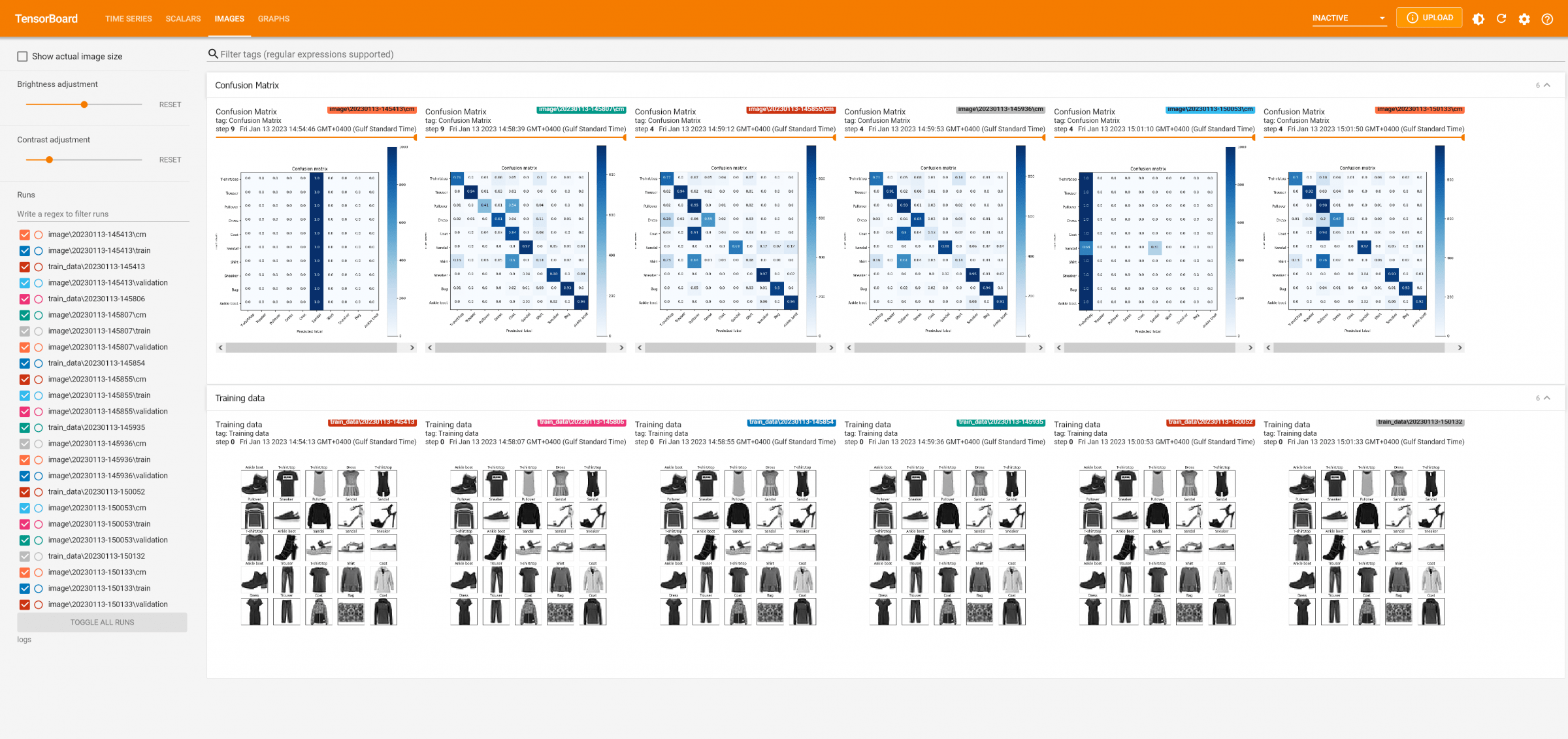
A simple image classification by Tensorflow and visualization by TensorBoard

Some of the features of TensorBoard include:

Scalar: visualizing scalar values such as accuracy, loss, or any other scalar values you want to track.
Histograms: visualizing the distribution of a Tensor over time.
Graphs: visualizing the computational graph of the model.
Images: visualizing image data.
Audio: visualizing audio data.
Text: visualizing text data.
Embeddings: visualizing high-dimensional data such as word embeddings.

TensorBoard also allows you to compare different runs of your model, and to compare the performance of different models. This can be useful for identifying patterns, trends, and other insights that can help you improve the performance of your models.